
§5–§9, §13 · method
The mathematics, live.
The full derivation behind the pricer, a worked example that reproduces its own numbers, the interactive pricer itself, and a live measurement of what it costs in accuracy.
§5
Mathematics of moment matching
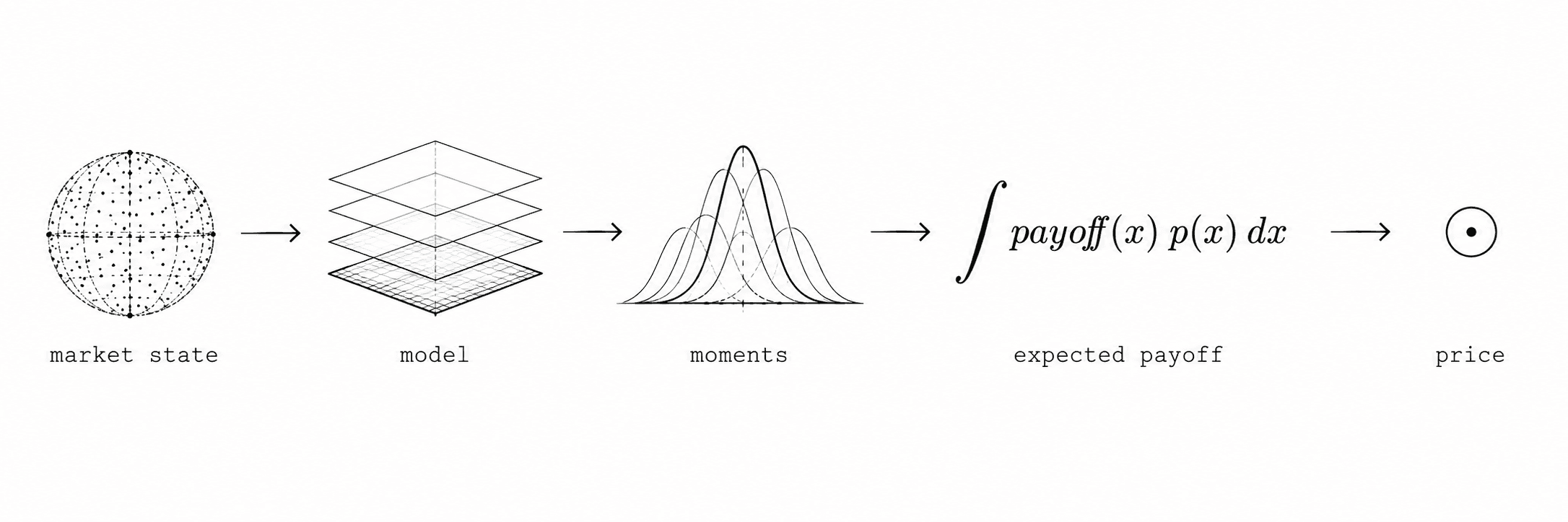
fig. 6 —The same pipeline as fig. 1, drawn out one stage further: market state, the GBM model, the two moments it implies, the expected-payoff integral against the matched proxy, and the resulting price.
The underlying is modeled as geometric Brownian motion under the risk-neutral measure, with cost of carry b = r − q. The averaging window is taken to run from now (t = 0) to expiry (t = T) — the natural setup for an on-chain engine reading a running oracle average.
GBM under the risk-neutral measure; W(t) is a standard Brownian motion.
The continuous-time analogue of the arithmetic average is A(T) = (1/T)∫₀ᵀ S(t) dt. Its first two moments follow from the moments of S(t) — no simulation required, because the integral of an expectation is the expectation of the integral.
First moment of the average. As bT → 0 this reduces to M₁ → S, its natural limit.
Second moment of the average — longer to state, but still closed-form; see the derivation below.
▸Show the derivation of M₁ and M₂
From (3), E[S(t)] = S·e^(bt), so by linearity of expectation and integration,
M₁ = E[(1/T)∫S(t)dt] = (1/T)∫S·e^(bt) dt = S·(e^(bT) − 1)/(bT).
For M₂ = E[A(T)²], write A(T)² as a double integral and push the expectation inside:
M₂ = (1/T²) ∫₀ᵀ∫₀ᵀ E[S(t)S(u)] dt du.
Under (3), for t ≤ u, Cov(W(t), W(u)) = t, which gives the product moment a closed form:
E[S(t)S(u)] = S²·exp( b(t+u) + σ²·min(t,u) ) = S²·exp( b(t+u) + σ²t ) for t ≤ u.
The region t ≤ u contributes half the square by symmetry, so M₂ = (2/T²)∫₀ᵀ∫₀ᵘ S²·e^(b(t+u)+σ²t) dt du. Evaluating this exponential double integral in closed form — routine but long — gives equation (5). The full algebra is carried out in Turnbull & Wakeman (1991) and reproduced in Haug (2007); it is not repeated here, but every step is an ordinary exponential integral, not an approximation in itself.
A lognormal distribution is fully determined by two parameters, so matching its mean and variance to M₁ and M₂ pins it down exactly:
Variance of the matched lognormal proxy, annualized.
Adjusted cost of carry, such that M₁ = S·exp(b_adj·T) exactly — this makes M₁ act as a forward price.
With the proxy’s forward (M₁) and volatility (σₐ) in hand, the call price follows from the standard Black-76 formula — exact for the proxy, approximate for the real average:
d₁ and d₂ as usual, with the matched forward M₁ and volatility σₐ in place of spot and σ. Φ is the standard normal CDF.
summary — the algorithm in four steps
- Read S, r, q from the oracle.
- Estimate σ from realized oracle history.
- Compute M₁, M₂ from (4)–(5); derive σₐ, b_adj from (6)–(7).
- Evaluate the closed form (8) — one evaluation, no iteration.
§6
Worked example
Every intermediate value below is computed by the same code that runs the live pricer in §7, for the scenario S = 100, K = 100, T = 1 year, σ = 60%, r = 4%, q = 0% — the pricer’s own defaults. Set it to the same values and it reproduces the last row exactly.
| quantity | meaning | value |
|---|---|---|
| b = r − q | cost of carry | 0.04 − 0.00 = 0.04 |
| e^(bT) | growth factor over T | e^0.04 = 1.040811 |
| M₁ (eq. 4) | first moment of the average | 100 · (1.040811 − 1) / 0.04 = 102.0269 |
| M₂ (eq. 5) | second moment of the average | 11 794.1707 |
| ln M₂ − 2 ln M₁ | matched log-variance · T | 0.124887 |
| σₐ (eq. 6) | matched volatility of the average | √0.124887 = 0.353394 (35.34%) |
| b_adj (eq. 7) | adjusted carry | ln(102.0269 / 100) = 0.020067 |
| d₁, d₂ (eq. 8) | standardized moneyness | d₁ = 0.233480, d₂ = −0.119914 |
| Φ(d₁), Φ(d₂) | standard normal CDF | 0.592305, 0.452276 |
| M₁Φ(d₁) − KΦ(d₂) | undiscounted expected payoff | 102.0269·0.592305 − 100·0.452276 = 15.2035 |
| e^(−rT) | discount factor | e^(−0.04) = 0.960789 |
| C (eq. 8) | price | 0.960789 · 15.2035 = 14.6074 |
notice —the matched volatility of the average, σₐ ≈ 35.3%, is well below the input spot volatility of 60%. This is not an error: averaging a path dampens its variance, and equation (6) captures that dampening arithmetically rather than by assumption.
§7
Live pricer
Arithmetic Asian call, evaluated by equation (8). All computation below runs locally in your browser — no API call, no server — using the same TypeScript module that the unit tests in the repository exercise. Change any input and the price recomputes deterministically. In production, S, r and q would be read from an oracle[1] rather than typed in.
| symbol | parameter | units |
|---|---|---|
| S | spot price, read from the oracle | quote currency |
| K | strike price | quote currency |
| T | time to expiry = length of the averaging window | years |
| σ | annualized volatility of the underlying | decimal, e.g. 0.6 = 60%/yr |
| r | continuously-compounded risk-free rate | decimal /yr |
| q | continuously-compounded dividend / carry yield | decimal /yr |
table 1 — inputs to price() and greeks()
instrument
Arithmetic-average Asian call
price
14.6074
delta
0.5806
vega (/1.00 vol)
23.0850
approximation notice
Price is a Turnbull–Wakeman moment-matched approximation, not an exact solution — no exact closed form exists for this payoff. Delta and vega are computed numerically, not in closed form — see §8. Approximation error is not quantified here in isolation; see §9 for a live comparison against a Monte Carlo reference.
fig. 5 —56 simulated GBM paths under the inputs above — illustration only, not the pricing method. Each path is colored by whether its own arithmetic average lands above (blue) or below (red) the strike K. Seeded from the input values rather than Math.random, so identical inputs always draw identical paths, and the shapes redraw instantly as you edit S, K, T, σ, r, or q above.
§8
Sensitivities: delta and vega
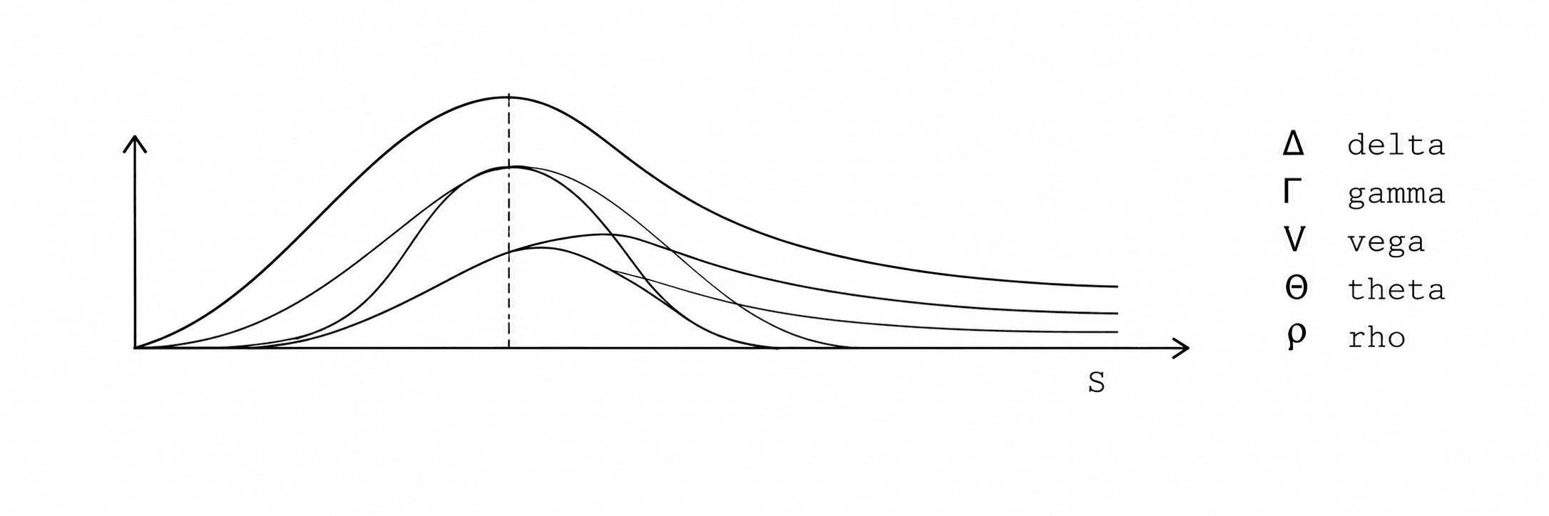
fig. 9 —The five standard Greeks, schematically, as functions of spot. This engine currently computes only Δ and vega (V) — Γ, Θ, and ρ are shown for context, not implemented here.
Equation (8) could be differentiated by hand with respect to S and σ — the chain rule through M₁, M₂, σₐ and d₁, d₂ is tedious but not hard. This engine doesn’t do that. Instead it treats price() as a black box and bumps it[5]: evaluate the price at S ± h, subtract, divide by 2h. The advantage is that the same two lines of code work for delta, for vega, and for any future pricing function dropped in to replace this one — the disadvantage is two extra price evaluations per Greek, and a small, tunable amount of finite-difference error on top of the model error already discussed in §3–§4.
Central finite-difference delta. h is a small bump in spot (10⁻⁴ of S in this implementation).
Central finite-difference vega. h is a small absolute bump in volatility (10⁻⁴ here).
| greek | h | C(x+h) | C(x−h) | result |
|---|---|---|---|---|
| Δ | 0.01 (= 10⁻⁴·S) | 14.613215 | 14.601602 | 0.580617 |
| vega | 0.0001 | 14.609716 | 14.605099 | 23.084970 |
table 2 — same scenario as §6 (S=100, K=100, T=1, σ=60%, r=4%, q=0%)
§9
Accuracy: error vs. compute
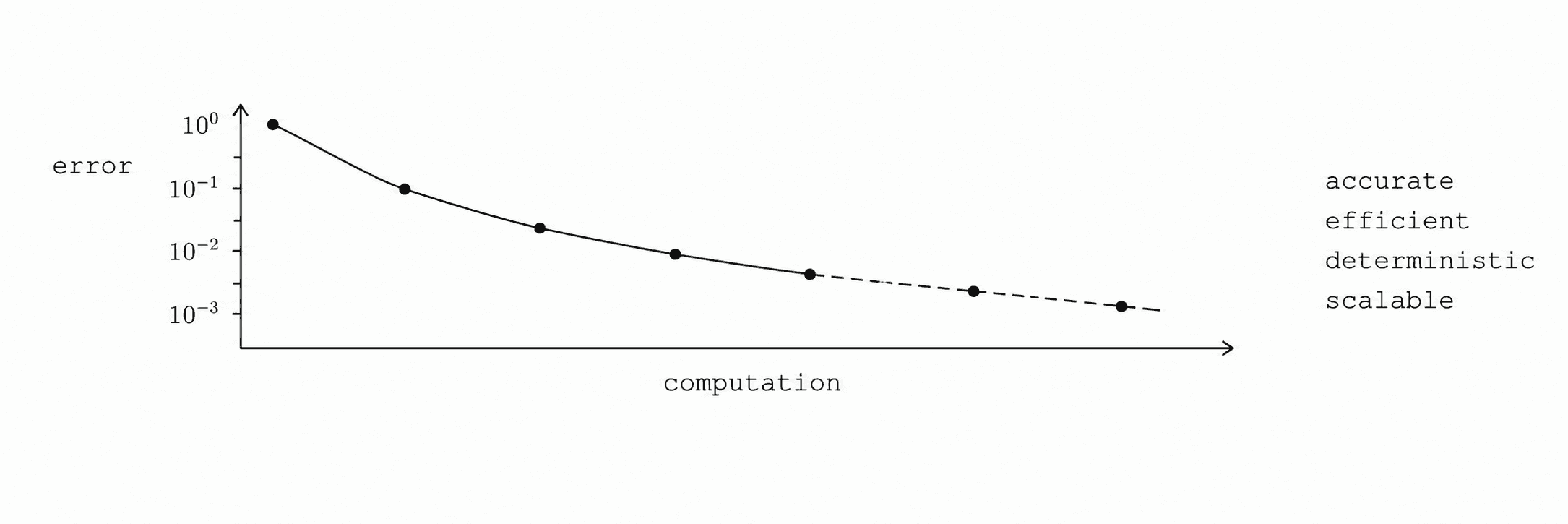
fig. 10 —The general shape of the argument in this paper, sketched — not this scenario’s actual numbers. The live-computed chart and table below are those numbers, for one specific case.
Computed live, in your browser, for one fixed scenario (S=100, K=100, T=1y, σ=60%, r=4%, q=0%). The 128- and 512-path Monte Carlo points are measured against a 6,000-path Monte Carlo reference[6]; the deterministic point is the Turnbull–Wakeman price measured against the same reference. This is one scenario, not a benchmark study — see §13 for what a real validation study requires.
computing…
Re-running changes the MC-128 and MC-512 points — that movement is sampling error. The deterministic point never moves, because it isn’t sampled.
§13
Validation methodology
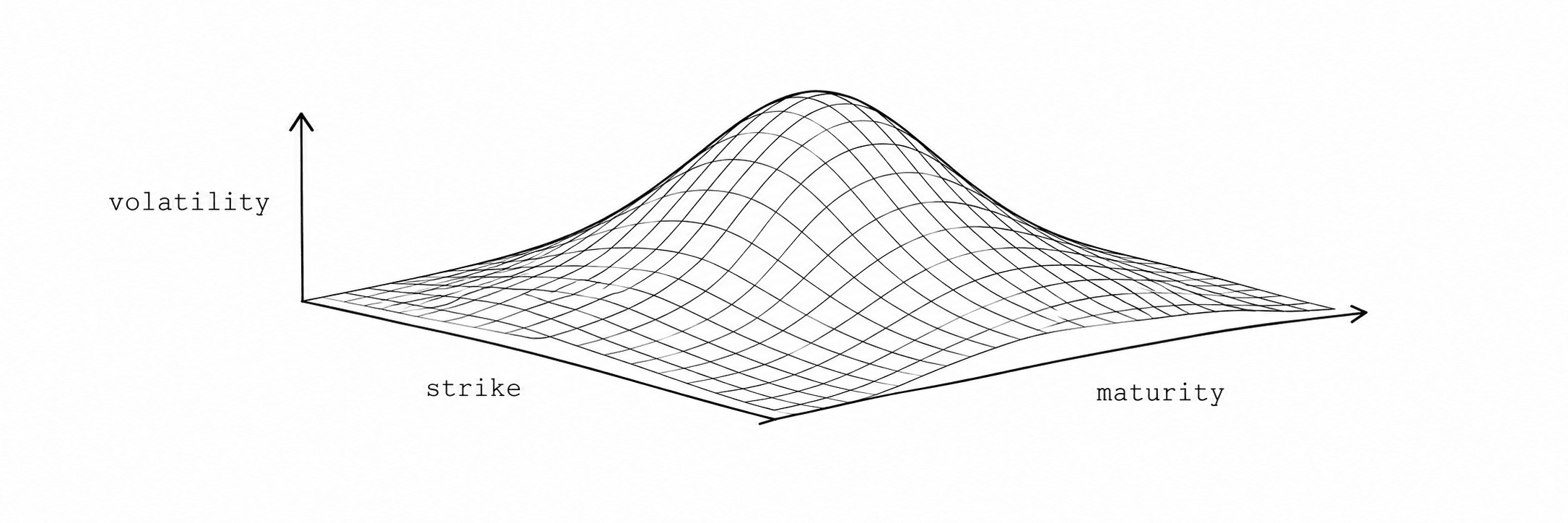
fig. 8 —Illustrative surface, not measured data: the shape an error-vs-(volatility, strike, maturity) surface is expected to take, given §10’s argument that model risk grows with σ√T. The actual surface is exactly what the sweep below would produce.
The comparison in §9 is one scenario, run live, for illustration. A real validation of the engine requires the Solidity implementation from §12 checked against a high-precision off-chain reference across a large, structured parameter sweep — not yet run. This section specifies that methodology in advance, so results, when they exist, have a pre-committed shape rather than being chosen after the fact.
metrics to be reported
- absolute pricing errorpending
- relative pricing errorpending
- worst-case errorpending
- gas / compute costpending
- error by volatilitypending
- error by maturitypending
- error by moneynesspending
references
- [1]Turnbull, S.M. and Wakeman, L.M. (1991). “A Quick Algorithm for Pricing European Average Options.” Journal of Financial and Quantitative Analysis, 26(3), 377–389. — source of the moment-matching approximation used throughout §5–§6.
- [2]Haug, E.G. (2007). The Complete Guide to Option Pricing Formulas, 2nd ed. McGraw-Hill. — exposition of the Turnbull–Wakeman formula this implementation follows.
- [3]Black, F. (1976). “The Pricing of Commodity Contracts.” Journal of Financial Economics, 3(1–2), 167–179. — source of the Black-76 forward-price form used in equation (8).
- [4]Kemna, A.G.Z. and Vorst, A.C.F. (1990). “A Pricing Method for Options Based on Average Asset Values.” Journal of Banking and Finance, 14(1), 109–129. — an earlier moment-matching approach to Asian options; related work, not the method used here.
- [5]Levy, E. (1992). “Pricing European Average Rate Currency Options.” Journal of International Money and Finance, 11(5), 474–491. — an alternative moment-matching formulation; related work, not the method used here.
- [6]Press, W.H., Teukolsky, S.A., Vetterling, W.T. and Flannery, B.P. (1992). Numerical Recipes in C, 2nd ed. Cambridge University Press, §6.2. — source of the erfc approximation used for the standard normal CDF.
reproduction
Everything on this page runs client-side, from the TypeScript source at src/lib/pricing/ — there is no server component and no API. §6 and §8’s tables are not typeset by hand: they are the output of that code for the stated inputs, and will match exactly if reproduced. §9 is the deliberate exception — it calls Math.random(), so its Monte Carlo columns are expected to differ, run to run; that difference is the subject of §3, not a bug in this page. A public code repository is planned but not yet published — see the footer.
notes
- [1]“Oracle” here means any on-chain contract that publishes a price other contracts can read in the same transaction — a Chainlink-style push feed, a Pyth-style pull feed, or a DEX TWAP. This project does not depend on, or specify, a particular oracle implementation. ↩
- [5]The finite-difference step sizes used here (10⁻⁴ of spot for delta, 10⁻⁴ absolute for vega) trade two error sources against each other: too large a step and the estimate picks up curvature (truncation error); too small a step and floating-point cancellation dominates (rounding error). These values were chosen empirically for double-precision arithmetic and have not been tuned per-instrument. ↩
- [6]The Monte Carlo reference in §9 discretely monitors the average at 32 equally spaced steps, which approximates the continuously-monitored average this engine assumes. That discretization is a second, separate source of error from the reference's own sampling error — with enough paths the reference converges to the discretely-monitored price, not necessarily to the continuous-average price. ↩